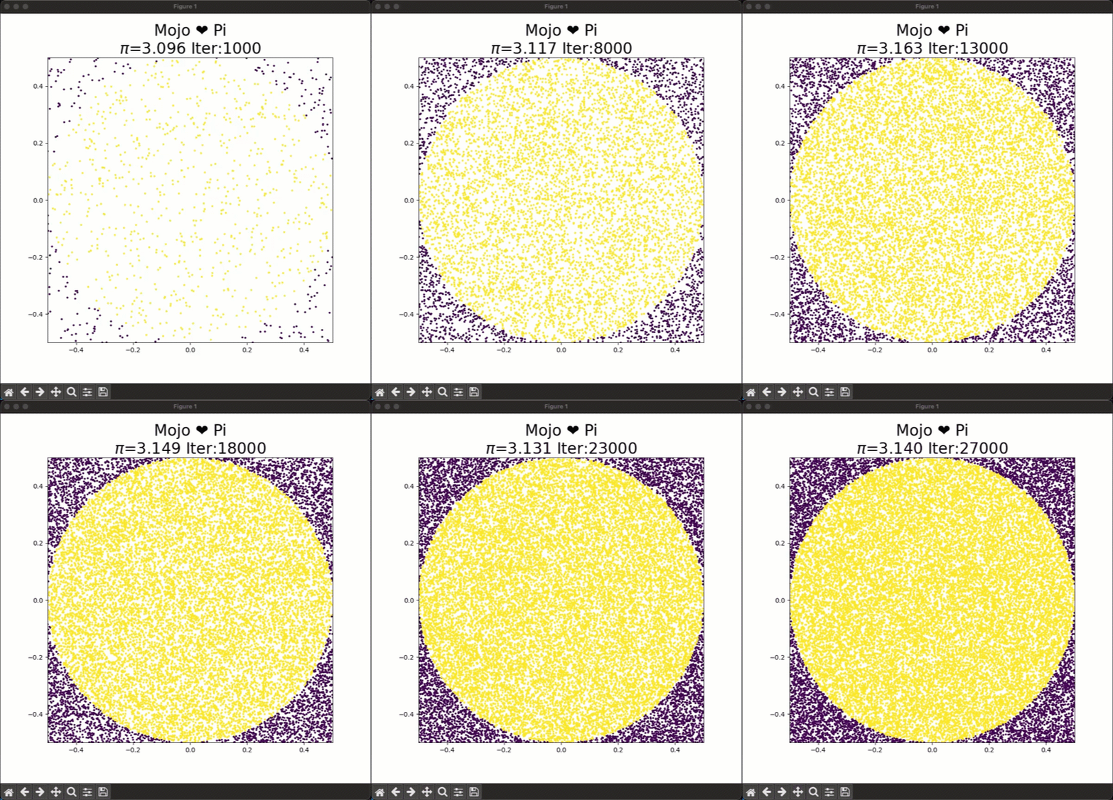
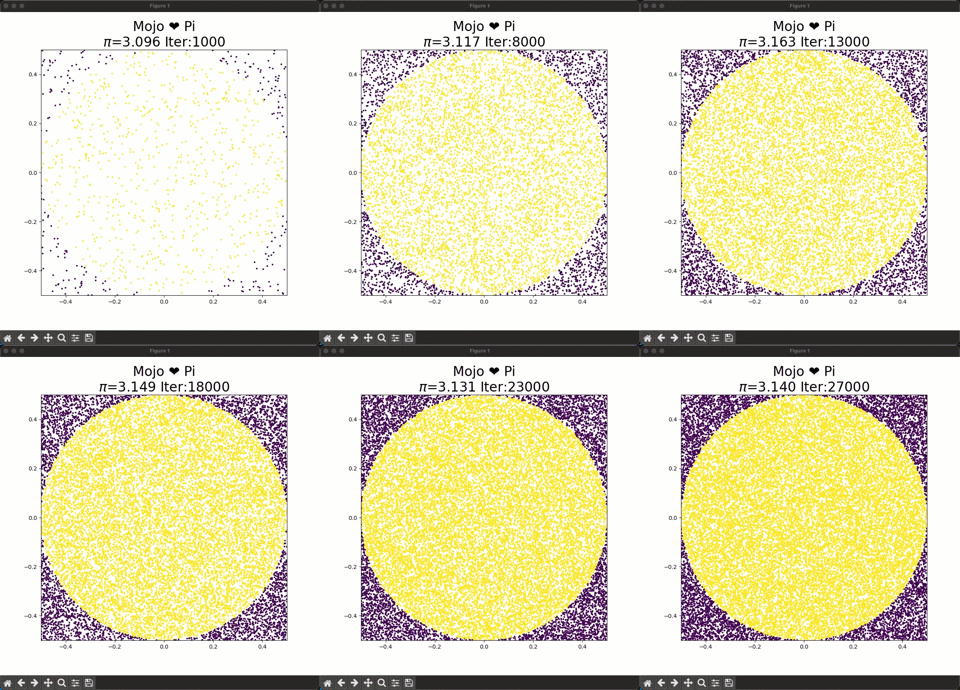
March 14th aka 3/14 or 3.14 is known as $\pi$ Day, and it honors the mathematical constant $\pi$ (pi), which represents the ratio of a circle's circumference to its diameter. On this special day, I wanted to dedicate a blog post to the beauty of mathematics, numerical methods, $\pi$, and Mojo. So join me on this journey as I implement a fast vectorized Monte Carlo approximation method of calculating $\pi$. Happy $\pi$ Day!

Approximating Pi

There are several methods for approximating $\pi$ including several Monte Carlo methods. Monte Carlo methods rely on repeated random sampling to obtain numerical results and rely on computation power to provide approximate solutions when solutions are hard to analyze mathematically. For this blog post, I chose one of the simplest Monte Carlo methods for approximating $\pi$. 

Consider a circle inscribed in a unit square, the ratio of the area of the square to area of the circle is ${\pi}/4$:

$\frac{Area-of-circle}{Area-of-square} = \frac{\pi * (0.5)^2}{1*1} = \frac{\pi}{4}$

To approximate the areas we can repeatedly sample from an uniform random distribution x, y $\in$ [-0.5,0.5] and place these dots on the square. The ratio of dots inside the circle to the total number of dots will approximately equal π/4. To calculate $\pi$ you have to calculate:

$4*\frac{dots-inside-circle}{dots-inside-square}$.

As you increase the number of dots the approximation for Pi gets closer to the true value, and you can see this in the animation at the top.

Approximating Pi in Mojo🔥

My goal with this blog post is to introduce you to some Mojo features as we implement this approach. The code for this blog post is available on GitHub. I’ll be building on the sample implementation of MojoArray I used in the Valentine’s day blog post. The core logic for pi calculation is as follows:

1. Randomly sample x and y coordinates from a uniform random distribution with upper and lower limits = [-0.5,0.5]
2. Calculate the magnitude of each dot using L2 norm
3. Get a list of dots whose magnitudes are less than equal to 0.5, which is the radius of the circle
4. Calculate $\pi$ with the formula $4*\frac{sum(inside-dots)}{N}$

The code for these steps are here:

For the above code to work, we have to add few additional functionality to MojoArray we implemented in the Valentine’s day blog post:

1. Get boolean array from greater than and less than equal operations using __gt__() and __le__() and convert this into float array so we can perform arithmetic operations on it
2. Support sum reduction, implemented in sum()

“Less than equal to” operations

Here I have a vectorized implementation of less than equal operations using SIMD types, that calculates the boolean response and then maps it into the default float representation of MojoArray (Float64). We need the float representation as the output to do a reduction and get the total number of dots in the next step. Note: I could have also used an integer representation, which will save some memory, but I chose the easy way out by using the default dtype MojoArray was initialized with.

 For __le__() the crux of the logic is in the following line:

In this line of code, we are operating on vectors of SIMD width for Float64 to speed up computation. First we load the vector and then do a “less than or equal to” comparison to return a boolean vector which contains True if it’s less than equal to val or False if it’s not. Then we use the select function to map the boolean vector to a floating point vector 1.0 (iters+1) or a 0.0 (iters) and save it in the new bool_float_array. We wrap this code in a closure and call vectorize which will automatically apply the operation to the entire MojoArray.

Calculating the sum reduction

After we have the floating point representation of the boolean array, we have to reduce it to a scalar by adding all the 1s to count the number of dots inside the circle. We do this in a vectorized way in the following function:

We allocate a sum vector of simd_width to save the intermediate sums, and in the vectorize_reduce function, we perform vectorized additions. Again, we wrap this code in a closure and call vectorize which will automatically apply the operation to the entire MojoArray. 

Finally we reduce the final vector s using the reduce_add() method.

Calculating Pi

Now we’re ready to taste some Pie 🥧😋, i mean Pi $\pi$. With our MojoArray data structure in place, we’re now ready to calculate Pi.

1. Define a large sample size with N
2. In a loop calculate Pi for different values of i from 0 to N in steps of 1000. For each i:
3. Create MojoArrays for x and y
4. Calculate radius r using L2 norm (aka euclidean distance, aka pythagoras theorem)
5. Get a list of inside dots that are <= 0.5
6. Calculate pi
7. Plot results using Python module Matplotlib
8. Loop till you reach N

The code for the main loop is here:

And the resulting animation:

Conclusion

Hope you enjoyed reading this blog post on how to calculate Pi in Mojo using Monte Carlo method. What better way to celebrate Pi day than by delving into the implementing approximation of pi while geeking out on Mojo🔥. You can find all the full implementation on GitHub.

While the implementation was elementary, my hope is that you can reuse some of the learnings in your own projects using Mojo. Download Mojo to run this example and share your feedback with us! Happy Pi Day! 

Here are some additional resources to get started. 

• Get started with downloading Mojo
• Head over to the docs to read the programming manual and learn about APIs
• Explore the examples on GitHub
• Join our Discord community
• Contribute to  discussions on the Mojo GitHub
• Read and subscribe to Modverse Newsletter 
• Read Mojo blog posts, watch developer videos and past live streams
• Report feedback, including issues on our GitHub tracker

Until next time🔥!